Buffer vs. image performance for applying filters to an image pyramid in OpenCL


When you have worked with images in OpenCL before, you may have wondered how to store them. Basically, we have the choice between using buffers or image objects. The later seems to be designed for that task, but what are the differences and how do they perform differently when applying a certain task? For a recent project, I needed to decide which storage type to use and I want to share the insights here. This is a follow-up article to my previous post where I already evaluated filter operations in OpenCL.

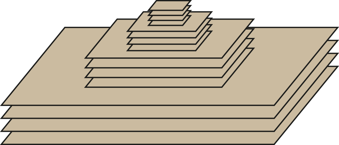
I did not only need to store plain images but rather a complete image pyramid, like visualized in the following figure, originating from a scale space. The pyramid consists of four octaves with four images each making up 16 levels in total. In each octave, the size of the images is always the same. With my used example image, the four images in the first octave have the size of the base image which is \(3866 \times 4320\) pixels. \(1933 \times 2160\) pixels are used in the second, \(966 \times 1080\) in the third and \(483 \times 540\) in the fourth octave making up a total of 88722000 pixels.

Image pyramid consisting of four octaves with four images each
Figure 1: Image pyramid consisting of four octaves with four images each. The image is half-sampled after each octave.

In order to measure the performance for the best storage types to use for the image pyramid, I applied image convolution with two derivative filters (Scharr filters) to the complete pyramid testing with the filter sizes of \(3 \times 3\), \(5 \times 5\), \(7 \times 7\) and \(9 \times 9\). I decided to assess four storage types for this task:

  • Buffer objects are basically one-dimensional arrays which can store any data you want. All pixel values of the image pyramid are stored as a one-dimensional array with a length of 88722000 in this case. This introduces overhead in the access logic, though, since the pyramid is by its nature not one-dimensional but rather three-dimensional with a non-uniform structure, i.e. not all images in the pyramid have the same size. I use a lookup table to minimize the overhead during computation. However, there is still the overhead for the programmer which needs to implement the logic.
  • Image buffer objects are created from buffers (so a cl::Buffer object is additionally necessary on the host side) and are offered by convenience to use a buffer which behaves like an image. However, it is very limited and can e.g. not be controlled by a sampler object. But it turns out that it is sometimes faster than buffers on my machine as we will see later. In theory, it would also be possible to use one-dimensional images (e.g. image1d_t in the kernel code) but this type of object is limited to the maximum possible width of a 2D image object (16384 on my machine) and hence not suitable to store an image pyramid with 88722000 pixels. Image buffers are not under this constraint but rather restricted by the CL_DEVICE_IMAGE_MAX_BUFFER_SIZE value (134217728 on my machine).
  • Images are a special data type in OpenCL which can be one-, two- and three-dimensional. The 16 levels of the image pyramid are stored as 16 image objects, e.g. as std::vector<cl::Image2D>. Handling of this object type is easiest for the programmer and as it will turn out is also very fast and I ended up using this storage type for my project.
  • Cubes are very similar to image types. They basically add a third dimension to the image objects. The idea here is that each octave, where all images have the same size, is stored in one cube resulting in four cubes in total. The overhead should be less for cubes than for images but I could not confirm this definitively in the benchmarks below hence I did not use this type.

The idea behind the four storage types is also visualized in the following figure.

Four different storage types (buffer, images and cubes) used in this benchmark
Figure 2: Four different storage types (buffer/image buffer, images and cubes) used in this benchmark. The first quads (buffers) represent pixels, the other images.

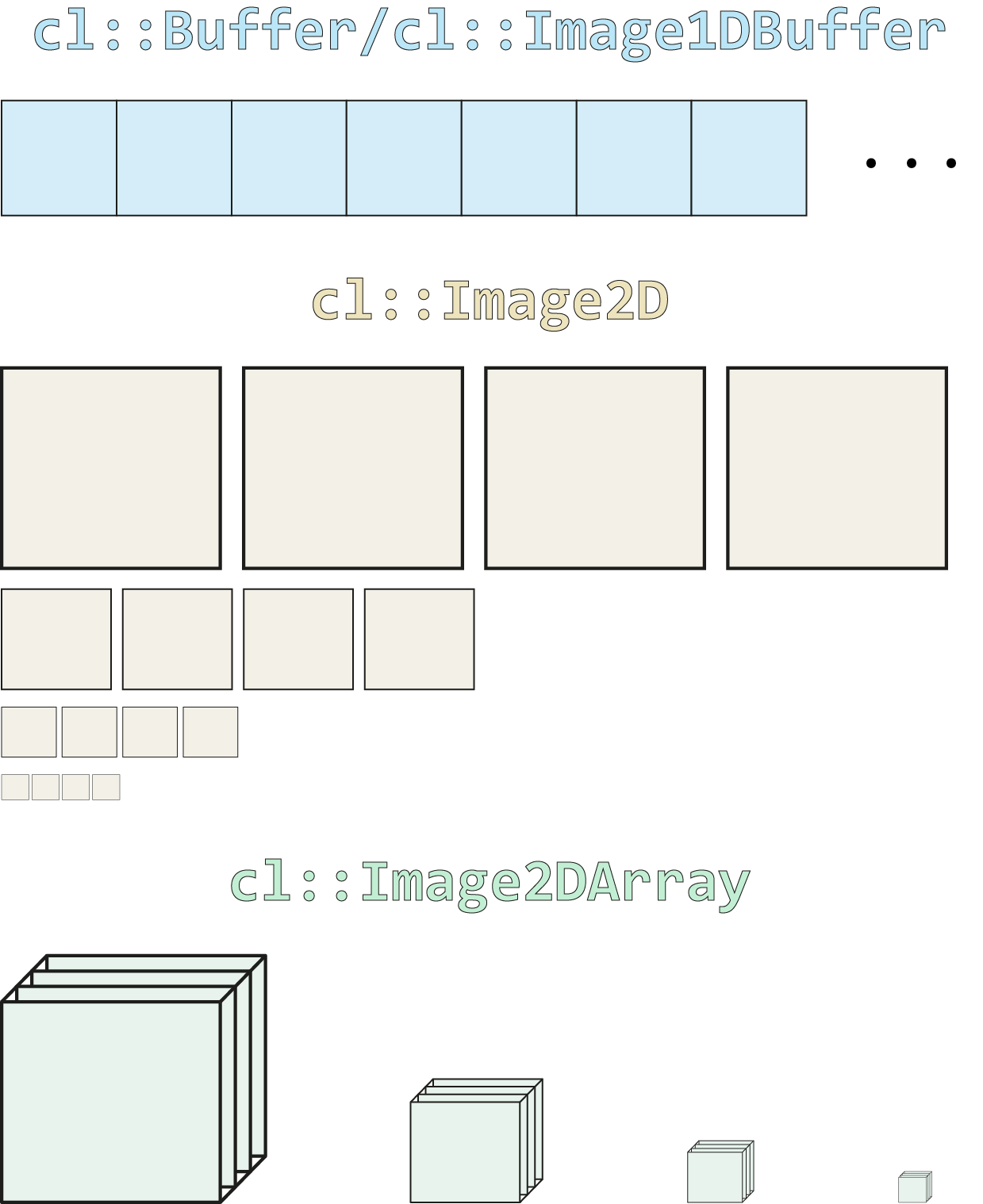
The four types and their properties are also summarized in the table below.

Storage type Host side type Kernel side type Kernel calls
Buffer cl::Buffer global float* 4
Image buffer cl::Image1DBuffer image1d_buffer_t 4
Images cl::Image2D image2d_t img 16
Cubes cl::Image2DArray image2d_array_t img 4

The column with the kernel calls denotes how often the OpenCL kernel must be executed in order to apply one filter to the complete image pyramid. Images need the most since the filter kernel must be applied to each image layer in the pyramid individually. The other types contain the notion of an octave in the pyramid and hence know that four images have the same size. It is, therefore, possible to apply the filter function to the complete octave at once.

Before diving into the benchmark though, I want to describe a bit the hardware details about the differences between buffers and images. Note that I use an AMD R9 290 @ 1.1 GHz GPU in the benchmark and hence concentrate only on the GCN architecture.

Buffer vs. images in the hardware context

It is not very easy to find detailed information about how the different storage types are handled by the hardware (or I am too stupid to search). But I will present my findings anyway.

The most important note is that image objects are treated as textures in the graphics pipeline. Remember that GPUs are designed for graphics tasks and the thing we do here in GPGPU with OpenCL is more the exception than the rule (even though it is an important field). Textures are a very important part of computer graphics and when you have ever developed your own (min)-game you know how fruitful this step is. As soon as textures are involved the whole scene does look suddenly much better than before. It is therefore only natural that the hardware has native support for it.

In computer graphics, a lot of tasks need to be done related to textures, e.g. texture mapping. This is the process where your images are mapped to the triangles in the scene. Hence, the hardware needs to load the necessary image pixels, maybe do some type conversion (e.g. float to int) or even compression (a lot of textures need a lot of space) and don't forget address calculations, interpolating as well as out-of border handling. To help with these tasks, the vendors add extra texture units which implement some of the logic in hardware. This is also visible in the block diagram of a compute unit of the AMD R9 290

As you can see, the transistors responsible for textures are located on the right side. There are four texture units (green horizontal bars) where each unit is made up of one filter unit and four address units. Why four times more address units than filter units? I don't know if this was the design choice but I would guess that this has something to do with bilinear interpolation where four pixels are needed to calculate one texel. It is also possible that this has something to do with latency hiding and hardware parallelism. Memory fetches may need a lot of time compared to the execution of ALU instructions in the SIMD units. In order to stay busy, the hardware executes multiple threads at once so that while one thread still waits for the data the others can already start with execution. But each thread needs data and must issue memory requests hence multiple store and load units are necessary. Note that these texture units are located on each compute unit and are not shared on a per-device basis. My device has 40 compute units so there are 160 texture units in total.

The address units take the requested pixel location, e.g. an \(x\) and \(y\) coordinate, and calculate the corresponding memory address. It could be possible that they do something like \(cols*y + x\) to calculate the address. When interpolation is used, the memory addresses for the surrounding pixels must be calculated as well. Anyway, requests to the memory system are issued and this involves the L1 cache (16 KB) next to the address units. This cache is sometimes also called the texture cache (since it holds texels).

Since the cache is shared between all wavefronts on the compute unit, it offers an automated performance gain when the wavefronts work on overlapping regions of the same data. E.g. in image convolution the pixels need to be accessed multiple times due to the incorporation of the neighbourhood. When the wavefronts on the compute unit process neighbouring image areas, this can speed up the execution since less data needs to be transferred from global to private memory. It is loaded directly from the cache instead.

There is also a global L2 texture cache with a size of 1 MB which is shared by all compute units on the device. Usually, the data is first loaded in the L2 cache before it is passed to the L1 caches of the compute units. In case of image convolution, the L2 cache may hold a larger portion of the image and each compute unit uses one part of this portion. But there is an overlap between the portions since pixels from the neighbourhood are fetched in the image convolution operation as well.

Buffers and image objects are also accessed differently from within OpenCL kernel code. Whereas a buffer is only a simple pointer and can be accessed as (note also how the address calculation is done in the kernel code and hence executed by the SIMD units)


kernel void buffer(global float* imgIn, global float* imgOut, const int imgWidth)
{
    const int x = get_global_id(0);
    const int y = get_global_id(1);
    float value = imgIn[imgWidth * y + x];
    //...
    imgOut[imgWidth * y + x] = value;
}

i.e. directly without limitations (it is just a one-dimensional array), image objects need special built-in functions to read and write values:


// CLK_ADDRESS_CLAMP_TO_EDGE = aaa|abcd|ddd
constant sampler_t sampler = CLK_NORMALIZED_COORDS_FALSE | CLK_ADDRESS_CLAMP_TO_EDGE | CLK_FILTER_NEAREST;

kernel void images(read_only image2d_t imgIn, write_only image2d_t imgOut)
{
    const int x = get_global_id(0);
    const int y = get_global_id(1);
    float value = read_imagef(imgIn, sampler, (int2)(x, y)).x;
    //...
    write_imagef(imgOut, (int2)(x, y), value);
}

So, the function read_imagef(image2d_t image, sampler_t sampler, int2 coordinates) is needed to access the pixels. This is necessary so that the hardware can optimize the code and make use of the texture units where the sampler is used to configure it. But how can the cool functions I promised before now be used in OpenCL or equivalently: how to set up the texture filter units to do what we want?

  • Interpolating: set the sampler to CLK_FILTER_LINEAR for bilinear and CLK_FILTER_NEAREST for nearest neighbour filtering. The additional texels are loaded automatically and the interpolated value is returned. If you need this interpolating functionality, you can also store other data than pixels in the image objects and get automatic interpolation.
  • Out-of-border handling: set the sampler e.g. to CLK_ADDRESS_CLAMP_TO_EDGE to repeat the last values or use one of the other constants. The modes are a bit limited when not using normalized coordinates, though; but still, better than nothing.
  • Type conversion: this is controlled by the used function in the kernel. Above read_imagef was used which returns a float value. Use e.g. read_imagei to return an int. Note that the functions in the kernel are independent of the real format set up on the host side.

How do buffer objects now differ? They don't use the texture units for a start since we do not provide a sampler object and do not use the built-in access functions. But they also use the cache hierarchy (bot L1 and L2) according to the docs. The programming guide by AMD states on page 9 “Actually, buffer reads may use L1 and L2. [...] In GCN devices, both reads and writes happen through L1 and L2.” and in the optimization guide on page 14 they claim further “The L1 and L2 read/write caches are constantly enabled. Read-only buffers can be cached in L1 and L2.”. This sounds for me that both caches are used for buffers as well but the benchmark results below suggest that a cache-friendly local work-group size seems to be important.

Regarding performance of the different memory locations, the general relationship is global > texture cache > local > private (cf. page 13ff of the optimization guide for some numbers). So even when image objects and hence texture cache is used, it may still be beneficial to explicitly cache data which is needed more than once by using the local data share (located in the centre in the block diagram). It is not surprising that global memory is the slowest and private memory the fastest. The trick is to reduce the time needed to transfer the data in the private registers of the SIMD units.

Implementation details

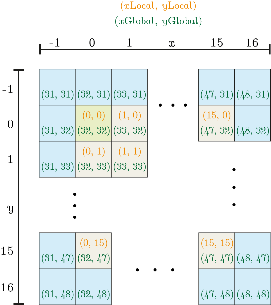
The buffer object is stored as a very long array in memory, but we still need to access locations in one of the images of the pyramid. But when we have only access to the 1D array from within the kernel, how do we write to a certain pixel location, let's say point \(p_1 = (10, 2)\) in level 9 of the pyramid? I decided to use a lookup table which is implemented as an array of structs defined as


struct Lookup
{
    int previousPixels;
    int imgWidth;
    int imgHeight;
};

The most important information is previousPixels which gives the number of pixels from all previous images and hence is the start offset for the buffer to find the pixel in the considered image. Helper functions to read and write to a certain pixel location can now be defined as


float readValue(float* img, constant struct Lookup* lookup, int level, int x, int y)
{
    return img[lookup[level].previousPixels + lookup[level].imgWidth * y + x];
}

void writeValue(float* img, constant struct Lookup* lookup, int level, int x, int y, float value)
{
    img[lookup[level].previousPixels + lookup[level].imgWidth * y + x] = value;
}

E.g. for \(p_1\) the memory address is calculated as lookup[8].previousPixels + lookup[8].966 /* = 3866 / 4 */ * 2 + 10. The lookup array is filled on the host side and transferred to the GPU as an argument to the filter kernel. The following snippet does the computation on the host side and includes an example.


/*
 * The following code generates a lookup table for images in a pyramid which are located as one long
 * buffer in memory (e.g. 400 MB data in memory). The goal is to provide an abstraction so that it is
 * possible to provide the level and the pixel location and retrieve the image value in return.
 *
 * Example:
 *  - original image width = 3866
 *  - original image height = 4320
 *  - image size in octave 0 = 3866 * 4320 = 16701120
 *  - image size in octave 1 = (3866 / 2) * (4320 / 2) = 4175280
 *  - image size in octave 2 = (3866 / 4) * (4320 / 4) = 1043820
 *  - number of octaves = 4
 *  - number of images per octave = 4
 *
 *  Number of pixels for image[8] (first image of octave 2):
 *  - pixels in previous octaves = 4 * 16701120 + 4 * 4175280 = 83505600
 *  - previous pixels for image[8] = 83505600
 *
 *  Number of pixels for image[9] (second image of octave 2):
 *  - pixels in previous octaves = 4 * 16701120 + 4 * 4175280 = 83505600
 *  - previous pixels for image[9] = 83505600 + 1043820 = 84549420
 */
locationLoopup.resize(pyramidSize);
int previousPixels = 0;
int octave = 0;
for (size_t i = 0; i < pyramidSize; ++i)
{
    locationLoopup[i].previousPixels = previousPixels;

    // Store size of current image
    locationLoopup[i].imgWidth = static_cast<int>(img.cols / pow(2.0, octave));
    locationLoopup[i].imgHeight = static_cast<int>(img.rows / pow(2.0, octave));

    // The previous pixels for the next iteration include the size of the current image
    previousPixels += locationLoopup[i].imgWidth * locationLoopup[i].imgHeight;

    if (i % 4 == 3)
    {
        ++octave;
    }
}

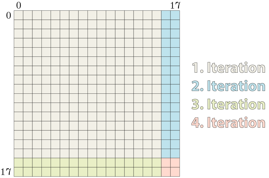
The same technique is used for the image buffers as well. When it comes to enqueue the kernel at the host side, the following code is executed for each octave.


//...
const size_t depth = 4;
const int base = octave * depth;    // octave is given as function argument
const size_t rows = lookup[base].imgHeight;
const size_t cols = lookup[base].imgWidth;

//...
const cl::NDRange offset(0, 0, base);
const cl::NDRange global(cols, rows, depth);
queue->enqueueNDRangeKernel(kernel, offset, global, local);

Note the used offset which stores the number of previous images (e.g. 8 in the octave = 2 iteration) and depth = 4 which makes this kernel a 3D problem: the filter is computed for all image pixels in all four images of the current octave.

The code for images and cubes is not very exciting, so I will not show any details for them. Check out the implementation if you want to know more.

Benchmark

It is now time to do some benchmarking. I start by testing a normal filter operation (called single in the related article). A short summary of the implementation is: unrolling and constant memory is used for the filter but no other optimizations. The first thing I want to test is the difference between the default local work-group size, i.e. setting the corresponding parameter to cl::NullRange, and the size manually to \(16 \times 16\). This is a common block size for an image patch computed by a work-group and is also the maximum possible size on my AMD R9 290 GPU. It turns out that this setting is quite crucial for buffers as you can see in the next figure.

Figure 3: Benchmark which tests the influence of the local work-group size (but not using local memory yet). Default settings (solid) are compared to a fixed size of \(16 \times 16\) (dashed). Note that this is the maximum possible size for a work-group on an AMD R9 290. Hover over the points to see the exact number. Click on the label at the top to hide/show a line (especially useful for the buffer to make space for the other lines). The mean values per size are averaged over 20 runs. Test suite used to produce these numbers is also available on GitHub

It really is important to manually set the local work-group size for buffers. Performance totally breaks for larger filters. The fact that a fixed size increases the speed that much is, I think, indeed evidence that buffers use the cache hierarchy. Otherwise, the local size shouldn't matter that much. But, there are still some differences compared to image buffers. Even though they also profit from a manually set work-group size, the effect is not that huge. Maybe the texture address units do some additional stuff not mentioned here which helps to increase cache performance. I don't think that it is related to some processing in the texture filter units since there is not much left. No type conversion must be done and a sampler can't be used for image buffers anyway. Additionally, the address calculation (\(cols*y + x\)) is done in both buffers inside the kernel and therefore executed by the SIMD units. Another possibility would be that the local work-group size is set differently for image buffers than for normal buffers. Unfortunately, I don't know of a way to extract this size when not set explicitly (the profiler just shows NULL).

If you compare the image buffers with one of the other image types (e.g. images), you see that image buffers are a bit slower. This is the effect of the missing sampler and the address calculation which needs to be done manually for image buffers. So, if possible, you should still prefer the normal image type over image buffers. But let me note that sometimes it is not possible or desired to work with 2D image objects. For example, let's say you have a point structure like


struct KeyPoint
{
    int octave;
    int level;
    float x;
    float y;
};

and you want to store a list of points which can be located anywhere in the image pyramid. Suppose further you want later (e.g. in a different kernel call) access the image pixels and its neighbours. Then you need to have access to the complete image pyramid inside the kernel and not only to a specific image. This is only possible when the pyramid is stored in an (image) buffer because then you can read pixels from all levels at once.

Another noticeable comparison is between images and cubes. First, the local work-group size does not play an important role in both cases. The differences here are negligible. It is likely that the hardware has more room for optimization since it knows which pixels in the 2D image plane are accessed. Remember that bot \(x\) and \(y\) are provided to the access functions. Second, cubes are consistently slower than images. Even though cubes can be executed with only 4 instead of 16 kernel calls and hence results in less communication with the driver and therefore less overhead. Maybe cubes are too large and stress the caches too much so that the benefit of the kernel calls are neutralized. Anyway, this is precisely the reason why I decided to use images and not cubes to store my pyramid.

The next thing I want to assess is the benefit of local memory. The following chart compares the results for fixed size work-groups from before with the case that always local memory is used (implementation details about how to use local memory for this task are shown in the filter evaluation article).

Figure 4: Benchmark which tests the usage of local memory. With local (solid) is compared against no usage of local memory (dashed). In both cases, the local work-group size is set to a fixed size of \(16 \times 16\). Note that the dashed values are the same as in the previous chart and are just shown again for comparison. Hover over the points to see the exact number. Click on the label at the top to hide/show a line. The mean values per size are averaged over 20 runs.

It is clear that local memory is beneficial for filter sizes \(\geq 5 \times 5\) regardless of the storage type. This is not surprising though since local memory is still faster than the L1 cache. Additionally, the L1 cache is smaller (16 KB L1 vs. 64 KB LDS), so it is to be expected that for larger filters performance decreases. For a filter of size \(3 \times 3\) the situation is not that clear. Sometimes it is faster and sometimes not. Don't forget that the manual caching with local memory does also introduce overhead. The data must be copied to the LDS and read back by the SIMD units. In general, I would say that it is not worth to use local memory for such a small filter.

Considering only the lines which use local memory, the result looks a bit messy. No clear winner and crossings all over again. I decided to use normal image types since they are easy to handle and offer full configuration via the sampler object. But I would also recommend that you test this on your own hardware. The results are very likely to differ.

Performance evaluation of image convolution with gradient filters in OpenCL


Filter operations are very common in computer vision applications and are often the first operations applied to an image. Blur, sharpen or gradient filters are common examples. Mathematically, the underlying operation is called convolution and already covered in a separate article. The good thing is that filter operations are very well suited for parallel computing and hence can be executed very fast on the GPU. I worked recently on a GPU-project were the filter operations made up the dominant part of the complete application and hence got first priority in the optimization phase of the project. In this article, I want to share some of the results.

First, a few words about GPU programming1. The GPU is very different from the CPU since it serves a completely different purpose (mainly gaming). This results in a completely different architecture and design principles. A GPU is a so-called throughput-oriented device where the goal is to execute many, many tasks concurrently on the processing units. Not only that a GPU has much more processing units than a CPU, it is also designed to leverage massive parallelism, e.g. by the concept of additional hardware threads per core. Just as a comparison: the CPU is a latency-oriented device. Its main goal is to execute a single task very fast, e.g. by introducing fast memory caching mechanism.

The demanding task for the developer is to keep the GPU busy. This is only possible by exploiting the parallelism of the application and optimize the code regarding this subject. One important factor, and as I now learned the important factor, which stalls the GPU is memory access. Since the GPU has a lot of processing units it needs also more memory to serve the units with data. Unlike to the CPU, it is under control of the developer where to store the memory which offers great flexibility and an additional degree of freedom in the optimization process. Badly designed memory transfers, e.g. by repeatedly copying data from the global to the private memory of the work-items, can take up most of the execution time.

As you may already have guessed from the title, I use OpenCL as a framework in version 2.0 and all the tests are run on an AMD R9 2902 @ 1.1 GHz GPU. Scharr filter (gradient filter) in the horizontal and vertical direction

\begin{equation} \label{eq:FilterOptimization_ScharrFilter} \partial_x = \begin{pmatrix} -3 & 0 & 3 \\ -10 & {\color{Aquamarine}0} & 10 \\ -3 & 0 & 3 \\ \end{pmatrix} \quad \text{and} \quad \partial_y = \begin{pmatrix} -3 & -10 & -3 \\ 0 & {\color{Aquamarine}0} & 0 \\ 3 & 10 & 3 \\ \end{pmatrix} \end{equation}

are used as filter kernel (centre position highlighted) and applied to an image pyramid consisting of four octaves with four images each3. Every benchmark measures how fast the two filters can be applied to the complete pyramid averaged over 20 runs. Note, that the creation of the pyramid (including the initial image transfer to the GPU) or the compilation time of the kernels is not included. I only want to measure the impact of the filter operation. Since the size of the filter is also very important, four different dimensions are used: \(3 \times 3\), \(5 \times 5\), \(7 \times 7\) and \(9 \times 9\). Filters larger than \(3 \times 3\) are basically \eqref{eq:FilterOptimization_ScharrFilter} scaled up but with slightly different numbers. In any case, there are only six non-zero entries. Filters are stored in float* arrays and the image itself is a grey-scale image converted to floating data type, i.e. the OpenCL data type image2d_t is used.

I want to assess the performance of filter operations in five test cases:

  1. Single: filter operation without further optimizations.
  2. Local: the image data is cached in local memory to exploit the fact that each pixel is needed multiple times.
  3. Separation: both filters in \eqref{eq:FilterOptimization_ScharrFilter} are linearly separable. In this case, it is possible to split up each filter in a horizontal and vertical vector and apply them to the image in two passes.
  4. Double: \(\partial_x\) and \(\partial_y\) are independent of each other. Since usually the response from both filters is needed and both are applied to the same image, it is possible to write an optimized kernel for that case.
  5. Predefined: Scharr filters are very common and it is likely that we need them multiple times. We could write a specialized kernel just for Scharr filters without the need to pass the filter as a parameter to the kernel. We can even go one step further and take the values of the filter into account, e.g. by omitting zero entries.

I don't have an extra case where I put the filter in constant memory since this is an optimization which I already implemented in the beginning (it is not very hard since the only thing to do is to declare the parameter pointing to the filer as constant float* filter), so the usage of constant memory is always included. Another common optimization is filter unrolling where the filter size must be known at compile time. The compiler can then produce code containing the complete filter loop as explicit steps without introducing the loop overhead (e.g. conditional checks if the loop has ended). Since this is also something where every test case benefits from, it is included, too.

Note also that these cases are not independent of each other. It is e.g. possible to use local memory and separate the filter. This makes testing a bit complicated since there are a lot of combinations possible. I start by considering each case separately and look at selected combinations at the end. All code which I used here for testing is also available on GitHub.

The next sections will cover each of the test cases in more detail, but the results are already shown in the next figure so that you can always come back here to compare the numbers.

Figure 1: Test results for the filter operations as mean value over 20 runs for different filter sizes. Hover over the points to see the exact number. Click on the label at the top to hide/show a line. Don't be too confident with the absolute speed values since they depend highly on the used hardware and maybe also other things like driver version, but the ordinal relationship should be a bit meaningful.

Single

The basic filter operation without any optimizations is implemented straightforwardly in OpenCL. We centre our Scharr filter at the current pixel location and then perform the convolution. The full code is shown as it serves as the basis for the other test cases.


/**
 * Calculates the filter sum at a specified pixel position. Supposed to be called from other kernels.
 * 
 * Additional parameters compared to the base function (filter_single_3x3):
 * @param coordBase pixel position to calculate the filter sum from
 * @return calculated filter sum
 */
float filter_sum_single_3x3(read_only image2d_t imgIn,
                            constant float* filterKernel,
                            const int2 coordBase,
                            const int border)
{
    float sum = 0.0);
    const int rows = get_image_height(imgIn);
    const int cols = get_image_width(imgIn);
    int2 coordCurrent;
    int2 coordBorder;
    float color;

    // Image patch is row-wise accessed
    // Filter kernel is centred in the middle
    #pragma unroll
    for (int y = -ROWS_HALF_3x3; y <= ROWS_HALF_3x3; ++y)       // Start at the top left corner of the filter
    {
        coordCurrent.y = coordBase.y + y;
        #pragma unroll
        for (int x = -COLS_HALF_3x3; x <= COLS_HALF_3x3; ++x)   // And end at the bottom right corner
        {
            coordCurrent.x = coordBase.x + x;
            coordBorder = borderCoordinate(coordCurrent, rows, cols, border);
            color = read_imagef(imgIn, sampler, coordBorder).x;

            const int idx = (y + ROWS_HALF_3x3) * COLS_3x3 + x + COLS_HALF_3x3;
            sum += color * filterKernel[idx];
        }
    }

    return sum;
}

/**
 * Filter kernel for a single filter supposed to be called from the host.
 * 
 * @param imgIn input image
 * @param imgOut image containing the filter response
 * @param filterKernel 1D array with the filter values. The filter is centred on the current pixel and the size of the filter must be odd
 * @param border int value which specifies how out-of-border accesses should be handled. The values correspond to the OpenCV border types
 */
kernel void filter_single_3x3(read_only image2d_t imgIn,
                              write_only image2d_t imgOut,
                              constant float* filterKernel,
                              const int border)
{
    int2 coordBase = (int2)(get_global_id(0), get_global_id(1));

    float sum = filter_sum_single_3x3(imgIn, filterKernel, coordBase, border);

    write_imagef(imgOut, coordBase, sum);
}

The sampler is a global object. Also, borderCoordinate() is a helper function to handle accesses outside the image border. Both definitions are not shown here and I refer to the full implementation (both are defined in filter.images.cl) for further interest, but it is not important here for the tests. We can call the filter_single_3x3() kernel from the host with the cl::NDRange set to the image size of the current level in the pyramid, e.g. something like


//...
const size_t rows = imgSrc.getImageInfo<CL_IMAGE_HEIGHT>();
const size_t cols = imgSrc.getImageInfo<CL_IMAGE_WIDTH>();

imgDst = std::make_shared<cl::Image2D>(*context, CL_MEM_READ_WRITE, cl::ImageFormat(CL_R, CL_FLOAT), cols, rows);

cl::Kernel kernel(*program, "filter_single_3x3");
kernel.setArg(0, imgSrc);
kernel.setArg(1, *imgDst);
kernel.setArg(2, bufferKernel1);    // {-3, 0, 3, -10, 0, 10, -3, 0, 3}
kernel.setArg(3, border);           // BORDER_REPLICATE (aaa|abcd|ddd)

const cl::NDRange global(cols, rows);
queue->enqueueNDRangeKernel(kernel, cl::NullRange, global, cl::NullRange);

The needed filter sizes need to be defined correctly, e.g.


#define COLS_3x3 3
#define COLS_HALF_3x3 1
#define ROWS_HALF_3x3 1

with the half versions calculated with int cast, i.e. \(rowsHalf = \left\lfloor \frac{rows}{2} \right\rfloor\). They need to be set as defines so that #pragma unroll can do its job. As you can see from the test results, this solution is not very fast compared to the others. This is good news since there is still room for optimizations.

Local

In the filter operation, each pixel is accessed multiple times by different work-items due to the incorporation of the neighbourhood in the convolution operation. It is not very efficient to transfer the data again and again from global to private memory since access to global memory is very slow. The idea is to cache the image's pixel values in local memory and access it from here. This reduces the need for global memory transfers significantly.

Local memory is attached to each compute unit on the GPU and is shared between work-groups. Work-groups on different compute units can't share the same data, so the caching is restricted to the current work-group. Since the work-group size is limited, e.g. to \(16 \times 16\) on the AMD R9 290 GPU, we need to split up the image into \(16 \times 16\) blocks. Each work-group must copy the parts of the image it needs into its own local memory. This would be easy if a work-group would only need to access data from its own \(16 \times 16\) image block. But the incorporation of the neighbourhood also holds for the border pixels, so we need to copy a bit more than \(16 \times 16\) pixels from the image depending on the filter size. E.g. for a \(3 \times 3\) filter a 1 px wide padding is needed.

Ok, we just need to copy a few more pixels, shouldn't be a problem, should it? It turns out that this is indeed a bit tricky. The problem is: which work-items in the work-group copy which pixels? We need to define a pattern and write it down as (messy) index calculation in code. To make things a bit simpler, consider the following example of a \(16 \times 16\) block which is located somewhere around the top left corner.

Example for the transfer from global to local memory with a 3 x 3 filter
Figure 2: Example for the transfer from global to local memory with a \(3 \times 3\) filter. The outer index (black) corresponds to the image access in the for loop of the next listing. Inside the pixels, the top index \({\color{Orange}(x_{local},y_{local})}\) shows the local id and the bottom index pair \({\color{Green}(x_{global},y_{global})}\) the global id used in this example. Blue pixels are needed for padding to allow correct filter calculations of the border pixels. The green pixel in the top left corner of the patch marks the base pixel.

First, note that the size of the local buffer must be large enough to cover all pixels shown. The idea is then to iterate over the local buffer (outer index), map the calculation relative to the base pixel and then copy the data according to the current outer pixel. Usually, this involves 4 iterations where we start with a \(16 \times 16\) block in the top left corner and move on in a zigzag fashion to gather the remaining pixels as shown in the following figure.

Access pattern of the 2-loop approach needs four iterations to transfer the image pixels from global to local memory for a 3 x 3 filter
Figure 3: Access pattern of the 2-loop approach which fills the local buffer in four iterations using a \(3 \times 3\) filter.

Except for the first iteration and not too large filter sizes, not all of the 256 work-items are busy during this calculation. Especially the fourth iteration where only 4 of the 256 work-items do something useful is not beautiful to look at4. But since the local buffer size does not map perfectly with the size of the work-group, this is unavoidable with this pattern. Implementing it results in:


/**
 * Calculates the filter sum using local memory at a specified pixel position. Supposed to be called from other kernels.
 * 
 * Additional parameters compared to the base function (filter_single_local_3x3):
 * @param coordBase pixel position to calculate the filter sum from
 * @return calculated filter sum
 */
float filter_sum_single_local_3x3(read_only image2d_t imgIn,
                                  constant float* filterKernel,
                                  int2 coordBase,
                                  const int border)
{
    const int rows = get_image_height(imgIn);
    const int cols = get_image_width(imgIn);

    // The exact size must be known at compile time (no dynamic memory allocation possible)
    // Adjust according to the highest needed filter size or set via compile parameter
    local float localBuffer[LOCAL_SIZE_COLS_3x3 * LOCAL_SIZE_ROWS_3x3];   // Allocate local buffer

    int xLocalId = get_local_id(0);
    int yLocalId = get_local_id(1);

    int xLocalSize = get_local_size(0);
    int yLocalSize = get_local_size(1);

    // The top left pixel in the current patch is the base for every work-item in the work-group
    int xBase = coordBase.x - xLocalId;
    int yBase = coordBase.y - yLocalId;

#if COLS_3x3 >= 9 || ROWS_3x3 >= 9
    /*
     * Copy the image patch including the padding from global to local memory. Consider for example a 2x2 patch with a padding of 1 px:
     * bbbb
     * bxxb
     * bxxb
     * bbbb
     * The following pattern fills the local buffer in 4 iterations with a local work-group size of 2x2
     * 1122
     * 1122
     * 3344
     * 3344
     * The number denotes the iteration when the corresponding buffer element is filled. Note that the local buffer is filled beginning in the top left corner (of the buffer)
     *
     * Less index calculation but more memory accesses, better for larger filter sizes
     */
    for (int y = yLocalId; y < yLocalSize + 2 * ROWS_HALF_3x3; y += yLocalSize)
    {
        for (int x = xLocalId; x < xLocalSize + 2 * COLS_HALF_3x3; x += xLocalSize)
        {
            // Coordinate from the image patch which must be stored in the current local buffer position
            int2 coordBorder = borderCoordinate((int2)(x - COLS_HALF_3x3 + xBase, y - ROWS_HALF_3x3 + yBase), rows, cols, border);
            localBuffer[y * LOCAL_SIZE_COLS_3x3 + x] = read_imagef(imgIn, sampler, coordBorder).x;   // Fill local buffer
        }
    }
#else
    /*
     * Copy the image patch including the padding from global to local memory. The local ID is mapped to the 1D index and this index is remapped to the size of the local buffer. It only needs 2 iterations
     *
     * More index calculations but less memory accesses, better for smaller filter sizes (a 9x9 filter is the first which needs 3 iterations)
     */
    for (int idx1D = yLocalId * xLocalSize + xLocalId; idx1D < (LOCAL_SIZE_COLS_3x3 * LOCAL_SIZE_ROWS_3x3); idx1D += xLocalSize * yLocalSize) {
        int x = idx1D % LOCAL_SIZE_COLS_3x3;
        int y = idx1D / LOCAL_SIZE_COLS_3x3;
        
        // Coordinate from the image patch which must be stored in the current local buffer position
        int2 coordBorder = borderCoordinate((int2)(x - COLS_HALF_3x3 + xBase, y - ROWS_HALF_3x3 + yBase), rows, cols, border);
        localBuffer[y * LOCAL_SIZE_COLS_3x3 + x] = read_imagef(imgIn, sampler, coordBorder).x;   // Fill local buffer
    }
#endif
        
    // Wait until the image patch is loaded in local memory
    work_group_barrier(CLK_LOCAL_MEM_FENCE);

    // The local buffer includes the padding but the relevant area is only the inner part
    // Note that the local buffer contains all pixels which are read but only the inner part contains pixels where an output value is written
    coordBase = (int2)(xLocalId + COLS_HALF_3x3, yLocalId + ROWS_HALF_3x3);
    int2 coordCurrent;
    float color;
    float sum = 0.0f;

    // Image patch is row-wise accessed
    #pragma unroll
    for (int y = -ROWS_HALF_3x3; y <= ROWS_HALF_3x3; ++y)
    {
        coordCurrent.y = coordBase.y + y;
        #pragma unroll
        for (int x = -COLS_HALF_3x3; x <= COLS_HALF_3x3; ++x)
        {
            coordCurrent.x = coordBase.x + x;
            color = localBuffer[coordCurrent.y * LOCAL_SIZE_COLS_3x3 + coordCurrent.x];    // Read from local buffer

            const int idx = (y + ROWS_HALF_3x3) * COLS_3x3 + x + COLS_HALF_3x3;
            sum += color * filterKernel[idx];
        }
    }

    return sum;
}

The relevant part is located at the lines 46–54. Notice how x - COLS_HALF_3x3 maps to the outer index shown in the example and when this is added to the base pixel we cover the complete local buffer. For example, the work-item \(w_1 = {\color{Orange}(0, 0)}\) executes the lines in its first iteration as


int2 coordBorder = borderCoordinate((int2)(0 - 1 + 32, 0 - 1 + 32) /* = (31, 31) */, rows, cols, border);
localBuffer[0 * 18 + 0] = read_imagef(imgIn, sampler, coordBorder).x;

which copies the top left pixel to the first element in the local buffer. Can you guess which second pixel the same work-item copies in its second iteration?5

When working with local buffers there is one caveat: the size of the buffer must be known at compile time and it is not possible to allocate it dynamically. This means that the defines


#define LOCAL_SIZE_COLS_3x3 18 // 16 + 2 * 1
#define LOCAL_SIZE_ROWS_3x3 18 // 16 + 2 * 1

must be set properly before using this function. This becomes less of a problem when loop unrolling is used (like here) since then the filter size must be known anyway.

Skip the second #else pragma for now and consider line 76ff where the base index is calculated. This adds the padding to the local id since we need only calculate the filter responses of the inner block (the padding pixels are only read, not written). For example, the work-item \(w_1\) sets this to


int2 coordBaseLocal = (int2)(0 + 1, 0 + 1) /* = (1, 1) */;

and accesses later the top left pixel in its first iteration (since the filter is centred at \({\color{Orange}(0, 0)}\))


// Image patch is row-wise accessed
#pragma unroll
for (int y = -1; y <= 1; ++y)
{
    coordCurrent.y = 1 + -1;
    #pragma unroll
    for (int x = -1; x <= 1; ++x)
    {
        coordCurrent.x = 1 + -1;
        float color = localBuffer[0 * 18 + 0];    // Read from local buffer

        const int idx = (-1 + 1) * 3 + -1 + 1;
        sum += color * filterKernel[0];
    }
}

The access pattern shown in the lines 46–54 has the disadvantage that it needs at least 4 iterations even though a \(3 \times 3\) filter can theoretically fetch all data in two iterations (256 inner pixels and \(16*1*4 + 1*1*4 = 68\) padding pixels). Therefore, I also implemented a different approach (lines 61–68). The idea here is to map the index range of the local ids of the \(16 \times 16\) block to a 1D index and then remap them back to the local buffer size. This is also visualized in the following figure.

Remapping of a 16 x 16 block to the local buffer size
Figure 4: Remapping of a \(16 \times 16\) block to the local buffer size of \(18 \times 18\) (\(3 \times 3\) filter). The block indices are mapped to the \(0, \ldots, 255\) 1D index range and remapped back to the indices of the \(18 \times 18\) local buffer size. In the first iteration the opaque pixels are loaded and in the second iteration the transparent pixels (remaining pixels).

For the work-item \(w_{18} = {\color{Orange}(1, 1)}\) lines 61–68 expand to


for (int idx1D = 1 * 16 + 1 /* = 17 */; idx1D < (18 * 18 /* = 324 */); idx1D += 16 * 16 /* = 256 */) {
    int x = 17 % 18 /* = 17 */;
    int y = 17 / 18 /* = 0 */;

    // Coordinate from the image patch which must be stored in the current local buffer position
    int2 coordBorder = borderCoordinate((int2)(17 - 1 + 32, 0 - 1 + 32) /* = (48, 31) */, rows, cols, border);
    localBuffer[0 * 18 + 17] = read_imagef(imgIn, sampler, coordBorder).x;   // Fill local buffer
}

and issues a copy operation for the top right pixel from global memory into the local buffer. Even though this approach results in fewer iterations it comes at the cost of higher index calculations. Comparing the two approaches shows only a little difference in the beginning.

Figure 5: Test results for two different patterns of how to copy the data from global to local memory as mean value over 20 runs for different filter sizes. The blue line shows the result using 2 for loops (lines 46–54) and the orange line denotes the results when using just 1 for loop but more index calculations (lines 61–68).

Only for a \(7 \times 7\) filter there is a small advantage of \(\approx 1.5\,\text{ms}\) for the index remapping approach. It is very noticeable though that a \(9 \times 9\) filter is much faster in the 2-loops approach. This is the first filter which needs 3 iterations in the remapping approach (256 inner pixels and \(16*4*4+4*4*4=320>256\)) and the critical point where the overhead of the index calculations gets higher than the cost of the additional iteration in the 2-loop approach.

Even though the difference is not huge, I decided to use the remapping approach for filter sizes up to \(7 \times 7\) and the 2-loop approach otherwise (hence the #if pragma).

Comparing the use of local memory with the other test cases shows that local memory gets more efficient with larger filter sizes. In the case of a \(3 \times 3\) filter the results are even a little bit worse due to the overhead of copying the data from global to local memory. But for the other filter sizes, this is definitively an optimization we should activate.

Separation

Separation is an optimization which does not work with every filter. To apply this technique, it must be possible to split up the filter in one column and one row vector so that their outer product results in the filter again, e.g. for a \(3 \times 3\) filter the equation

\begin{align*} H &= \fvec{a} \cdot \fvec{b} \\ \begin{pmatrix} h_{11} & h_{12} & h_{13} \\ h_{21} & h_{22} & h_{23} \\ h_{31} & h_{32} & h_{33} \\ \end{pmatrix} &= \begin{pmatrix} a_1 \\ a_2 \\ a_3 \\ \end{pmatrix} \cdot \begin{pmatrix} b_1 & b_2 & b_3 \\ \end{pmatrix} \end{align*}

must hold. Luckily, this is true for our Scharr filter

\begin{align*} \partial_x &= \fvec{\partial}_{x_1} \cdot \fvec{\partial}_{x_1} \\ \begin{pmatrix} -3 & 0 & 3 \\ -10 & 0 & 10 \\ -3 & 0 & 3 \\ \end{pmatrix} &= \begin{pmatrix} -3 \\ -10 \\ -3 \\ \end{pmatrix} \cdot \begin{pmatrix} 1 & 0 & -1 \\ \end{pmatrix}. \end{align*}

How does this help us? Well, we can use this when performing the convolution operation with the image \(I\)

\begin{equation*} I * \partial_x = I * \fvec{\partial}_{x_1} * \fvec{\partial}_{x_2} = I * \fvec{\partial}_{x_2} * \fvec{\partial}_{x_1}. \end{equation*}

So, we can perform two convolutions instead of one and the order doesn't matter. This is interesting because we now perform two convolutions with a \(3 \times 1\) respectively a \(1 \times 3\) filter instead of one convolution with a \(3 \times 3\) filter. The benefit may be not so apparent for such a small filter but for larger filters, this gives us the opportunity to save a lot of computations. However, we also increase the memory consumption due to the need for a temporary image which is especially crucial on GPUs, as we will see.

But first, let's look at a small example. For this, consider the following definition of \(I\)

\begin{equation*} I = \begin{pmatrix} 0 & 1 & 0 & 1 \\ 2 & 2 & 0 & 0 \\ 0 & {\color{Aquamarine}3} & 1 & 0 \\ 0 & 1 & 0 & 0 \\ \end{pmatrix} \end{equation*}

where the convolution at the highlighted position is calculated as (note that the filter is swapped in the convolution operation)

\begin{equation*} (I * \partial_x)(2, 3) = 2 \cdot 3 + (-10) \cdot 1 = -4. \end{equation*}

To achieve the same result with separation we also need the horizontal neighbours of our element and apply the column-vector

\begin{align*} (I * \fvec{\partial}_{x_1})(1, 3) &= 2 \cdot (-3) + 0 \cdot (-10) + 0 \cdot (-3) = -6 \\ (I * \fvec{\partial}_{x_1})(2, 3) &= 2 \cdot (-3) + 3 \cdot (-10) + 1 \cdot (-3) = -39 \\ (I * \fvec{\partial}_{x_1})(3, 3) &= 0 \cdot (-3) + 1 \cdot (-10) + 0 \cdot (-3) = -10. \end{align*}

These are our temporary values where we would need a temporary image with the same size as the original image during the filter process. Next, apply the column vector on the previous results

\begin{equation*} \left( (I * \fvec{\partial}_{x_1}) * \fvec{\partial}_{x_2} \right)(2, 3) = (-6) \cdot (-1) + (-39) \cdot 0 + (-10) \cdot 1 = -4 \end{equation*}

and we get indeed the same result. If you want to see the full example, check out the attached Mathematica notebook.

The kernel code which implements separate filter convolution is not too different from the single approach. It is basically the same function, just using different defines


#define COLS_1x3 3
#define COLS_HALF_1x3 1
#define ROWS_1x3 1
#define ROWS_HALF_1x3 0

and adjust the names in the kernel definition accordingly


float filter_sum_single_1x3(read_only image2d_t imgIn,
                            constant float* filterKernel,
                            const int2 coordBase,
                            const int border)
{
    //...
    #pragma unroll
    for (int y = -ROWS_HALF_1x3; y <= ROWS_HALF_1x3; ++y)       // Start at the top left corner of the filter
    {
        coordCurrent.y = coordBase.y + y;
        #pragma unroll
        for (int x = -COLS_HALF_1x3; x <= COLS_HALF_1x3; ++x)   // And end at the bottom right corner
        {
            //...
            const int idx = (y + ROWS_HALF_1x3) * COLS_1x3 + x + COLS_HALF_1x3;
            sum += color * filterKernel[idx];
        }
    }

    return sum;
}

But from the host side, we need to call two kernels, e.g. something like


//...
cl::Image2D imgTmp(*context, CL_MEM_READ_WRITE, cl::ImageFormat(CL_R, CL_FLOAT), cols, rows);
imgDst = std::make_shared<cl::Image2D>(*context, CL_MEM_READ_WRITE, cl::ImageFormat(CL_R, CL_FLOAT), cols, rows);

cl::Kernel kernelX(*program, "filter_single_1x3");
kernelX.setArg(0, imgSrc);
kernelX.setArg(1, imgTmp);
kernelX.setArg(2, bufferKernelSeparation1A);    // (-3, -10, -3)^T
kernelX.setArg(3, border);

cl::Kernel kernelY(*program, "filter_single_3x1");
kernelY.setArg(0, imgTmp);
kernelY.setArg(1, *imgDst);
kernelY.setArg(2, bufferKernelSeparation1B);    // (1, 0, -1)
kernelY.setArg(3, border);

const cl::NDRange global(cols, rows);
queue->enqueueNDRangeKernel(kernelX, cl::NullRange, global);
queue->enqueueNDRangeKernel(kernelY, cl::NullRange, global);

Note the temporary image imgTmp which serves as output in the first call and as input in the second call. Beside that also two filters are needed at the host side (bufferKernelSeparation1A respectively bufferKernelSeparation1A) there is nothing special here.

If you look at the test results, you see that this approach performs not very well. For a \(3 \times 3\) filter it turns out that this is even a really bad idea since it produces the worst results from all. Even when things get better for larger filter sizes (which is expected) the results are not overwhelming. The main problem here is the need for an additional temporary image. We need as much as the size of the complete image as additional memory. What is more, we have more memory transfers: in the first run the data is transferred from global to private memory, the temporary response calculated and stored back in global memory. In the next run, the data is transferred again from global to private memory to calculate the final response which is, again, stored back in global memory. Since memory transfers from global to private memory are very costly on the GPU this back and forth introduces an immense overhead and this overhead manifests itself in the bad results.

Another thing I noticed here is that the range of values is very high (remember that the test results show only the mean value over 20 runs). This can be seen by considering a box-whisker plot of the data as in the following figure.

Figure 6: Test results for the separation test case shown as box-whisker plot for different filter sizes. The whiskers are set depending on the interquartile range, e.g. for the top whisker: \(q_{75} + 1.5 \cdot (q_{75} - q_{25})\) if an outlier exists. Disable the outlier in the legend to see the box-whisker plots in more detail.

Especially for the \(3 \times 3\) filter the range is really immense with outliers around 500 ms (half a second!). This really breaks performance and may be another symptom of the temporary image. I did not notice such behaviour for the other test cases.

I recently worked on a project where I needed a lot of filter operations which were, theoretically, all separable with sizes up to \(9 \times 9\). In the beginning, I used only separable filters without special testing. Later in the optimization phase of the project, I did some benchmarking (the results you are currently reading) and omitted separable filters completely as a consequence. This was a huge performance gain for my program. So, be careful with separable filters and test if they really speed up your application.

Double

Suppose you want to calculate the magnitude of the image gradients \(\left\| \nabla I \right\|\) (which is indeed a common task). Then both filters of \eqref{eq:FilterOptimization_ScharrFilter} need to be applied to the image and a task graph could look as follows.

Task graph to calculate the magnitude of the image gradients
Figure 7: Task graph to calculate the magnitude of the image gradients.

As you can see, the two filter responses can be calculated independently from each other. What is more: they both use the same image as input. We can exploit this fact and write a specialized kernel which calculates two filter responses at the same time.


float2 filter_sum_double_3x3(read_only image2d_t imgIn,
                             constant float* filterKernel1,
                             constant float* filterKernel2,
                             const int2 coordBase,
                             const int border)
{
    float2 sum = (float2)(0.0f, 0.0f);
    const int rows = get_image_height(imgIn);
    const int cols = get_image_width(imgIn);
    int2 coordCurrent;
    int2 coordBorder;
    float color;

    // Image patch is row-wise accessed
    // Filter kernel is centred in the middle
    #pragma unroll
    for (int y = -ROWS_HALF_3x3; y <= ROWS_HALF_3x3; ++y)       // Start at the top left corner of the filter
    {
        coordCurrent.y = coordBase.y + y;
        #pragma unroll
        for (int x = -COLS_HALF_3x3; x <= COLS_HALF_3x3; ++x)   // And end at the bottom right corner
        {
            coordCurrent.x = coordBase.x + x;
            coordBorder = borderCoordinate(coordCurrent, rows, cols, border);
            color = read_imagef(imgIn, sampler, coordBorder).x;

            const int idx = (y + ROWS_HALF_3x3) * COLS_3x3 + x + COLS_HALF_3x3;
            sum.x += color * filterKernel1[idx];
            sum.y += color * filterKernel2[idx];
        }
    }

    return sum;
}

kernel void filter_double_3x3(read_only image2d_t imgIn,
                              write_only image2d_t imgOut1,
                              write_only image2d_t imgOut2,
                              constant float* filterKernel1,
                              constant float* filterKernel2,
                              const int border)
{
    int2 coordBase = (int2)(get_global_id(0), get_global_id(1));

    float2 sum = filter_sum_double_3x3(imgIn, filterKernel1, filterKernel2, coordBase, border);

    write_imagef(imgOut1, coordBase, sum.x);
    write_imagef(imgOut2, coordBase, sum.y);
}

The filter_sum_double_3x3() function now takes two filter definitions as a parameter (lines 2–3) and returns both responses in a float2 variable which are saved in the two output images (lines 47–48). There is not more about it and it is not surprising that this test case outperforms the single approach. Of course, this works only with filters which do not need to be calculated sequentially.

Predefined

When we already know the precise filter definition like in \eqref{eq:FilterOptimization_ScharrFilter} we could use the information and write a kernel which is specialized for this filter. We don't have to pass the filter definition as an argument anymore and, more importantly, it is now possible to optimize based on the concrete filter values. In case of the Scharr filter, we can exploit the fact that we have three zero entries. There is no point in multiplying these entries with the image value or even loading the affected image pixels into the private memory of the work-item. An optimized kernel for \(\partial_x\) may look like


float filter_sum_single_Gx_3x3(read_only image2d_t imgIn,
                               const int2 coordBase,
                               const int border)
{
    float sum = 0.0f;
    const int rows = get_image_height(imgIn);
    const int cols = get_image_width(imgIn);
    int2 coordCurrent;
    int2 coordBorder;
    float color;

	coordCurrent.y = coordBase.y + -1;
	coordCurrent.x = coordBase.x + -1;
	coordBorder = borderCoordinate(coordCurrent, rows, cols, border);
	color = read_imagef(imgIn, sampler, coordBorder).x;
	sum += color * -3.0f;
	coordCurrent.x = coordBase.x + 1;
	coordBorder = borderCoordinate(coordCurrent, rows, cols, border);
	color = read_imagef(imgIn, sampler, coordBorder).x;
	sum += color * 3.0f;
	coordCurrent.y = coordBase.y;
	coordCurrent.x = coordBase.x + -1;
	coordBorder = borderCoordinate(coordCurrent, rows, cols, border);
	color = read_imagef(imgIn, sampler, coordBorder).x;
	sum += color * -10.0f;
	coordCurrent.x = coordBase.x + 1;
	coordBorder = borderCoordinate(coordCurrent, rows, cols, border);
	color = read_imagef(imgIn, sampler, coordBorder).x;
	sum += color * 10.0f;
	coordCurrent.y = coordBase.y + 1;
	coordCurrent.x = coordBase.x + -1;
	coordBorder = borderCoordinate(coordCurrent, rows, cols, border);
	color = read_imagef(imgIn, sampler, coordBorder).x;
	sum += color * -3.0f;
	coordCurrent.x = coordBase.x + 1;
	coordBorder = borderCoordinate(coordCurrent, rows, cols, border);
	color = read_imagef(imgIn, sampler, coordBorder).x;
	sum += color * 3.0f;

    return sum;
}

This is probably one of the most explicit forms possible. No for loops anymore, every operation is written down and the filter values are simple literals6. As you may have noticed, only six image values are loaded instead of nine as before. This limits memory transfer down to its minimum.

The benchmark results show that the approach performs very well and is relatively independent of the filter size. This is not surprising though since also larger Scharr filters have only six non-zero entries.

Selected combinations

Testing combinations of the approaches shown so far can easily turn into an endless story since so many combinations are possible. To keep things simple, I want to focus on three different questions:

  1. Does local memory also help to improve in the double approach? Would be weird if not.
  2. How does the double approach perform with predefined filters?
  3. Does local memory help with predefined filters?

As you can see, I already abandoned separate filters since their behaviour is just not appropriate for my application. The following chart contains a few more results to answer the questions.

Figure 8: Test results for combined test cases as mean value over 20 runs for different filter sizes. Hover over the points to see the exact number. Click on the label at the top to hide/show a line. Dotted lines correspond to the first question, dashed lines to the second and solid and dashed lines to the third.

As expected, the double approach does also benefit from local memory and works well with predefined filters. No surprises here. But note that local memory does not work well together with predefined filters, neither in the single nor in the double approach. Of course, since only six image values are loaded regardless of the filter size a huge difference is not to be expected. But it is interesting that the results with local memory are even worse (in both cases).

After all this testing, are there some general rules to infer? If you ask...

  • Whenever possible, calculate the response of two filters at the same time using the double approach.
  • If you know the exact filter definition in advance, write a specialized kernel just for that filter but test if using local memory speeds up your application.
  • In all other common cases make sure to use local memory for filter sizes \(> 3 \times 3\).
  • Don't forget that all results are highly application-, hardware- and software-specific. Take the time and test it on your own hardware and in your scenario.

List of attached files:


1. The intention of this article is not to give an introduction to GPU programming with OpenCL in general. I assume that you are already familiar with the basic concepts. Some keywords you should be familiar with: global, local, private and constant memory; compute unit, work-item and work-groups. As an introduction to this topic, I can recommend the book Heterogeneous Computing with OpenCL 2.0 (first edition) by David Kaeli et al.
2. It might be interesting to look at the block diagram of this device.
3. The image resolutions are \(3866 \times 4320\) for all four images in the first octave, \(1933 \times 2160\) in the second, \(966 \times 1080\) in the third and \(483 \times 540\) in the fourth octave (so, 88722000 pixels in total).
4. Since 64 threads of a wavefront execute the code in lockstep this means that 60 threads execute nothing useful.
5. Since we add the work-group size (16) to \(x\) after the first iteration, we get the new coordinates \((16 - 1 + 32, 0 - 1 + 32) = (47, 31)\).
6. From a code quality point of view, this is a nightmare since the code is very hard to maintain. However, I have not written it down manually; it is generated by a Perl script.

Addressing mode of sampler objects for image types in OpenCL reviewed


When working with image objects in OpenCL (e.g. image2d_t) special image functions like read_imagef must be used for accessing the individual pixels. One of the parameters, beside the image object and the coordinates, is a sampler_t object. This object defines the details about the image access. One detail is what should happen if coordinates are accessed which are out of the image boundaries. Several addressing modes can be used and this article discussed the difference on a small example.

If you are familiar with OpenCV's border types, you know that there are many ways to handle out of border accesses. Unfortunately, in OpenCL 2.0 the possible modes are much more limited. What is more, some of the addressing modes are limited to normalized coordinates \(\left([0;1[\right)\) only. The following table lists the addressing modes I tested here (cf. the documentation for the full description).

Addressing mode Example Normalized only? OpenCV's counterpart
CLK_ADDRESS_MIRRORED_REPEAT cba|abcd|dcb yes cv::BORDER_REFLECT
CLK_ADDRESS_REPEAT bcd|abcd|abc yes cv::BORDER_WRAP
CLK_ADDRESS_CLAMP_TO_EDGE aaa|abcd|ddd no cv::BORDER_REPLICATE
CLK_ADDRESS_CLAMP 000|abcd|000 no cv::BORDER_CONSTANT

The example column is already the result from my test program since the official documentation lacks an example here. In my test project (GitHub) I used a 1D image object with ten values incrementing from 1 to 10, i.e. a vector defined as


std::vector<float> dataIn = { 1, 2, 3, 4, 5, 6, 7, 8, 9, 10 };

For simplicity, I used a global size of exactly 1 work item and the following kernel code:


kernel void sampler_test(read_only image1d_t imgIn, write_only image1d_t imgOut, const int sizeIn, sampler_t sampler, global float* coords)
{
    int j = 0;                              // Index to access the output image
    for (int i = - sizeIn/2; i < sizeIn + sizeIn/2 + 1; ++i)
    {
        float coordIn = i / (float)sizeIn;  // Normalized coordinates in the range [-0.5;1.5] in steps of 0.1
        float color = read_imagef(imgIn, sampler, coordIn).x;

        coords[j] = coordIn;
        write_imagef(imgOut, j, color);     // The accessed color is just written to the output image
        j++;
    }
}

So, I access the coordinates in the range \([-0.5;1.5]\) in steps of 0.1 leading to 21 values in total. This results in five accesses outside the image on the left side, one access exactly at 1.0 and five more outside accesses on the right side. The fact that the access to 1.0 results already in a mode dependent value is indeed an indicator for the \([0;1[\) range (note that the right side is not included) of the normalized coordinates. The output of the test program running on an AMD R9 290 GPU device and on an Intel CPU device together with the differences:

            
            Platforms
                    0: Intel(R) OpenCL - OpenCL 1.2
                    1: Experimental OpenCL 2.1 CPU Only Platform - OpenCL 2.1
                    2: AMD Accelerated Parallel Processing - OpenCL 2.0 AMD-APP (2348.3)
            Choose platform: 2
            Devices on platform AMD Accelerated Parallel Processing
                    0: Hawaii - OpenCL 2.0 AMD-APP (2348.3)
                    1: Intel(R) Core(TM) i7-5820K CPU @ 3.30GHz - OpenCL 1.2 AMD-APP (2348.3)
            Choose device: 0
              coords | MIRRORED_REPEAT | REPEAT | CLAMP_TO_EDGE | CLAMP
            ---------|-----------------|--------|---------------|------
            -0.50000 |               5 |      6 |             1 |     0
            -0.40000 |               4 |      7 |             1 |     0
            -0.30000 |               3 |      8 |             1 |     0
            -0.20000 |               2 |      9 |             1 |     0
            -0.10000 |               1 |     10 |             1 |     0
             0.00000 |               1 |      1 |             1 |     1
             0.10000 |               2 |      2 |             2 |     2
             0.20000 |               3 |      3 |             3 |     3
             0.30000 |               4 |      4 |             4 |     4
             0.40000 |               5 |      5 |             5 |     5
             0.50000 |               6 |      6 |             6 |     6
             0.60000 |               7 |      7 |             7 |     7
             0.70000 |               8 |      8 |             8 |     8
             0.80000 |               9 |      9 |             9 |     9
             0.90000 |              10 |     10 |            10 |    10
             1.00000 |              10 |      1 |            10 |     0
             1.10000 |               9 |      2 |            10 |     0
             1.20000 |               8 |      3 |            10 |     0
             1.30000 |               7 |      4 |            10 |     0
             1.40000 |               6 |      5 |            10 |     0
             1.50000 |               5 |      6 |            10 |     0


            Platforms
                    0: Intel(R) OpenCL - OpenCL 1.2
                    1: Experimental OpenCL 2.1 CPU Only Platform - OpenCL 2.1
                    2: AMD Accelerated Parallel Processing - OpenCL 2.0 AMD-APP (2348.3)
            Choose platform: 1
            Devices on platform Experimental OpenCL 2.1 CPU Only Platform
                    0: Intel(R) Core(TM) i7-5820K CPU @ 3.30GHz - OpenCL 2.1 (Build 18)
            Choose device: 0
              coords | MIRRORED_REPEAT | REPEAT | CLAMP_TO_EDGE | CLAMP
            ---------|-----------------|--------|---------------|------
            -0.50000 |               6 |      6 |             1 |     0
            -0.40000 |               5 |      7 |             1 |     0
            -0.30000 |               4 |      8 |             1 |     0
            -0.20000 |               3 |      9 |             1 |     0
            -0.10000 |               2 |     10 |             1 |     0
             0.00000 |               1 |      1 |             1 |     1
             0.10000 |               2 |      2 |             2 |     2
             0.20000 |               3 |      3 |             3 |     3
             0.30000 |               4 |      4 |             4 |     4
             0.40000 |               5 |      5 |             5 |     5
             0.50000 |               6 |      6 |             6 |     6
             0.60000 |               7 |      7 |             7 |     7
             0.70000 |               8 |      8 |             8 |     8
             0.80000 |               9 |      9 |             9 |     9
             0.90000 |              10 |     10 |            10 |    10
             1.00000 |              10 |      1 |            10 |     0
             1.10000 |              10 |      2 |            10 |     0
             1.20000 |               8 |      3 |            10 |     0
             1.30000 |               8 |      3 |            10 |     0
             1.40000 |               7 |      4 |            10 |     0
             1.50000 |               6 |      6 |            10 |     0
            
            
AMD → Intel RENAMED
@@ -1,23 +1,23 @@
1
  coords | MIRRORED_REPEAT | REPEAT | CLAMP_TO_EDGE | CLAMP
2
  ---------|-----------------|--------|---------------|------
3
- -0.50000 | 5 | 6 | 1 | 0
4
- -0.40000 | 4 | 7 | 1 | 0
5
- -0.30000 | 3 | 8 | 1 | 0
6
- -0.20000 | 2 | 9 | 1 | 0
7
- -0.10000 | 1 | 10 | 1 | 0
8
  0.00000 | 1 | 1 | 1 | 1
9
  0.10000 | 2 | 2 | 2 | 2
10
  0.20000 | 3 | 3 | 3 | 3
11
  0.30000 | 4 | 4 | 4 | 4
12
  0.40000 | 5 | 5 | 5 | 5
13
  0.50000 | 6 | 6 | 6 | 6
14
  0.60000 | 7 | 7 | 7 | 7
15
  0.70000 | 8 | 8 | 8 | 8
16
  0.80000 | 9 | 9 | 9 | 9
17
  0.90000 | 10 | 10 | 10 | 10
18
  1.00000 | 10 | 1 | 10 | 0
19
- 1.10000 | 9 | 2 | 10 | 0
20
  1.20000 | 8 | 3 | 10 | 0
21
- 1.30000 | 7 | 4 | 10 | 0
22
- 1.40000 | 6 | 5 | 10 | 0
23
- 1.50000 | 5 | 6 | 10 | 0
1
  coords | MIRRORED_REPEAT | REPEAT | CLAMP_TO_EDGE | CLAMP
2
  ---------|-----------------|--------|---------------|------
3
+ -0.50000 | 6 | 6 | 1 | 0
4
+ -0.40000 | 5 | 7 | 1 | 0
5
+ -0.30000 | 4 | 8 | 1 | 0
6
+ -0.20000 | 3 | 9 | 1 | 0
7
+ -0.10000 | 2 | 10 | 1 | 0
8
  0.00000 | 1 | 1 | 1 | 1
9
  0.10000 | 2 | 2 | 2 | 2
10
  0.20000 | 3 | 3 | 3 | 3
11
  0.30000 | 4 | 4 | 4 | 4
12
  0.40000 | 5 | 5 | 5 | 5
13
  0.50000 | 6 | 6 | 6 | 6
14
  0.60000 | 7 | 7 | 7 | 7
15
  0.70000 | 8 | 8 | 8 | 8
16
  0.80000 | 9 | 9 | 9 | 9
17
  0.90000 | 10 | 10 | 10 | 10
18
  1.00000 | 10 | 1 | 10 | 0
19
+ 1.10000 | 10 | 2 | 10 | 0
20
  1.20000 | 8 | 3 | 10 | 0
21
+ 1.30000 | 8 | 3 | 10 | 0
22
+ 1.40000 | 7 | 4 | 10 | 0
23
+ 1.50000 | 6 | 6 | 10 | 0

Interestingly, the two devices produce slightly different values for the CLK_ADDRESS_MIRRORED_REPEAT and CLK_ADDRESS_REPEAT modes. I am not sure why this happens, but the AMD output seems more reasonable to me.